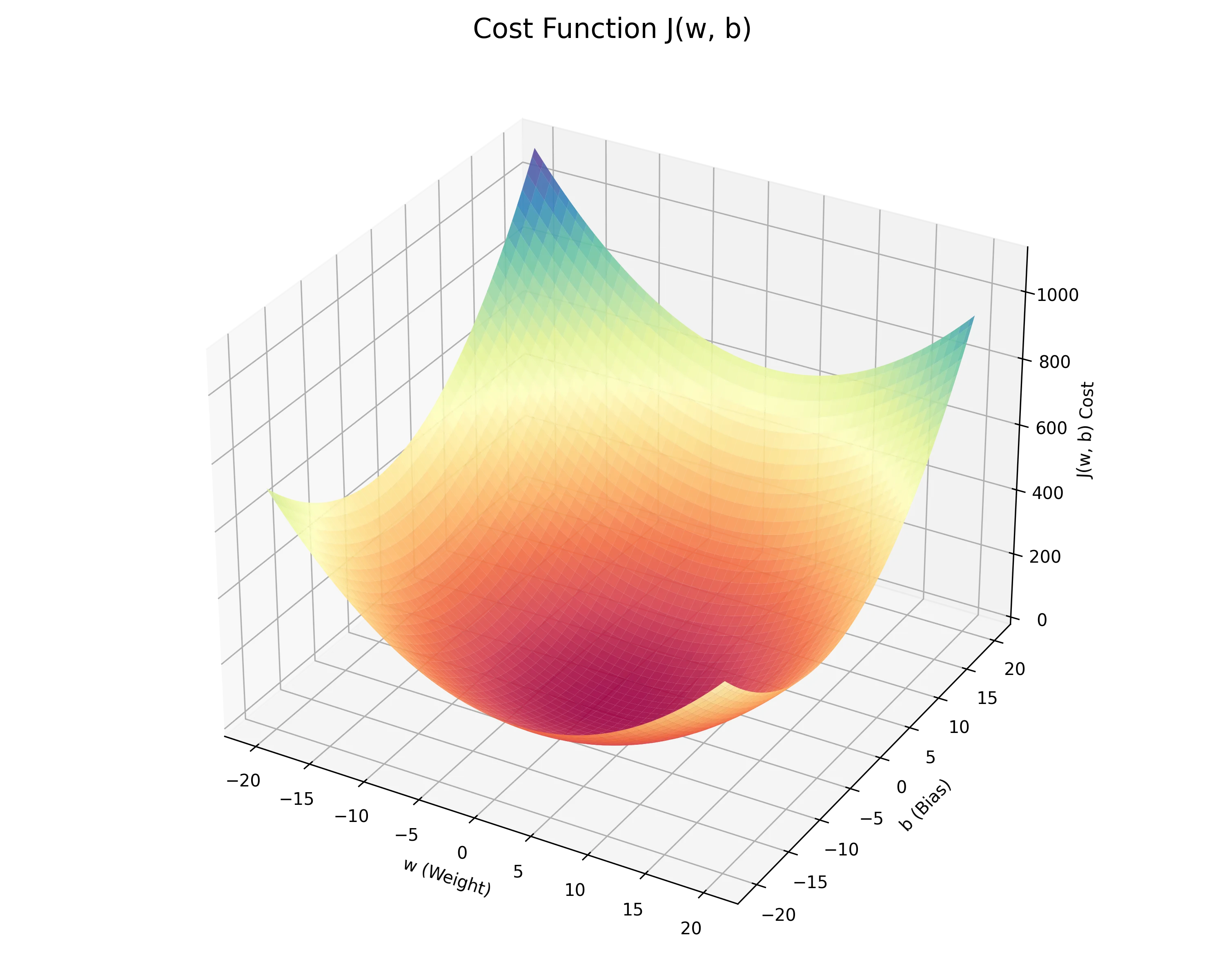
The Engine of Optimization

In machine learning, training a model means finding the best parameters (weights and biases) that allow the model to make accurate predictions. To measure “how accurate” our predictions are, we use a Cost Function.

The cost function is the mathematical compass that guides our optimization algorithms, such as Gradient Descent, toward the optimal parameters.

The Mean Squared Error (MSE)

For linear regression, the most common cost function is the Mean Squared Error (MSE). It measures the average of the squares of the errors—that is, the average squared difference between the estimated values and the actual true values.

Let $f_{w,b}(x^{(i)})$ be our model’s prediction for the $i$-th example, and $y^{(i)}$ be the actual true label. The MSE cost function $J(w, b)$ is defined as:

$$J(w, b) = \frac{1}{2m} \sum_{i=1}^{m} \left( f_{w,b}(x^{(i)}) - y^{(i)} \right)^2$$

Where:

• $m$ is the total number of training examples.
• $w$ is the weight parameter.
• $b$ is the bias parameter.
• $f_{w,b}(x) = wx + b$ is the linear model.

Geometric Interpretation

When we plot the cost function $J(w, b)$ against its parameters $w$ and $b$, we get a 3D surface. For linear regression using MSE, this surface is always a convex “bowl” shape.

This geometry is critical. Because it is convex, it guarantees that there is only one global minimum. No matter where we initialize our parameters on this surface, Gradient Descent will always roll down into the same global minimum—the absolute bottom of the bowl—representing the optimal fit.

Matrix Formulation (Vectorized)

For a technically accurate and computationally efficient implementation, the cost function is often expressed in its matrix form. This allows us to leverage optimized linear algebra libraries like NumPy.

Let $X$ be the design matrix of shape $(m, n+1)$, where each row is a training example (with a bias term $x_0=1$), $y$ be the target vector of shape $(m, 1)$, and $\theta$ be the parameter vector containing weights and bias of shape $(n+1, 1)$.

The predicted values are given by $\hat{y} = X\theta$. The MSE cost function in vectorized form is:

$$J(\theta) = \frac{1}{2m} (X\theta - y)^T (X\theta - y)$$

This elegant matrix equation computes the exact same squared errors as the summation loop but executes exponentially faster on modern hardware by utilizing SIMD instructions and GPU acceleration.

Gradient Descent

The algorithm used to find this minimum is Gradient Descent, which iteratively updates the parameters:

$$w = w - \alpha \frac{\partial J(w,b)}{\partial w}$$ $$b = b - \alpha \frac{\partial J(w,b)}{\partial b}$$

Where $\alpha$ is the learning rate, controlling the size of the steps we take down the hill. By computing the partial derivatives, the algorithm knows exactly which direction points “downhill”, systematically minimizing our error until the model is perfectly optimized.